Pulse Types¶

A standard gamma-ray burst looks like this

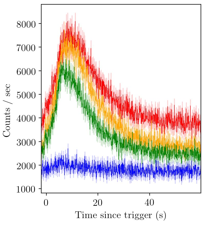
BATSE trigger 7475¶

Gaussian pulse¶

A simple pulse parameterisation one might imagine is a Gaussian, like those used to model emission lines in eg. quasar spectra. The equation for a Gaussian pulse is:

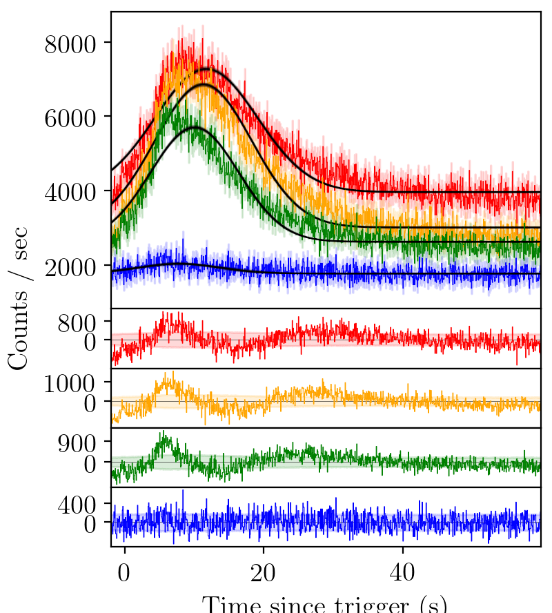
\[S(t|A,\Delta,\sigma) = A \exp \left[ \frac{\left( t - \Delta \right)^2}{2\sigma^2} \right]\]

BATSE trigger 7475 with gaussian fit¶

However, we can immediately see that such a pulse parameterisation does not catch the fast rise of the GRB pulse, nor the slow decay. The residuals have consistent structure.

FRED pulse¶

The standard pulse parameterisation used to model gamma-ray bursts is a fast-rise exponential-decay (FRED) curve.

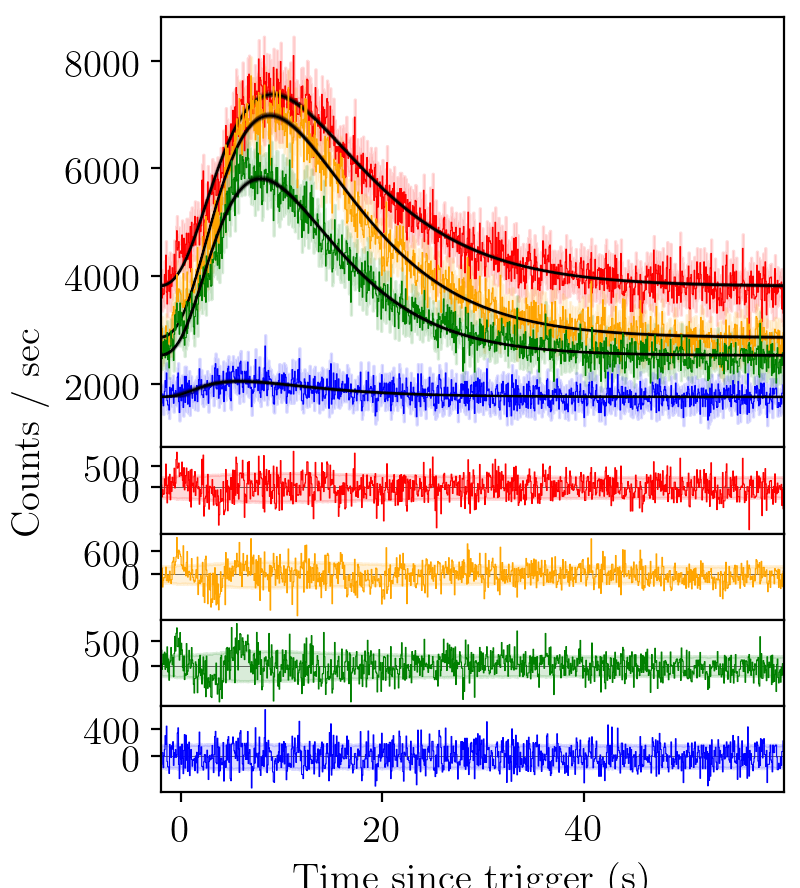
\[S(t|A,\Delta,\tau,\xi) = A \exp \left[ - \xi \left( \frac{t - \Delta}{\tau} + \frac{\tau}{t-\Delta} \right) \right]\]

BATSE trigger 7475 with FRED fit¶

The fit is better than a Gaussian, but again there is structure un-accounted for in the residuals.

FRED-X pulse¶

We try again with an extended fast-rise exponential-decay model, FRED-X.

\[S(t|A,\Delta,\tau,\xi,\gamma,\nu) = A \exp \left[ -\xi^\gamma \left(\frac{t - \Delta}{\tau}\right)^\gamma - \xi^\nu \left(\frac{\tau}{t-\Delta}\right)^\nu\right]\]

BATSE trigger 7475 with FRED-X fit¶

Again, an element of structure in the residual persists.

Sine-Gaussian residual¶

We use a sine-gaussian residual function to account for these residuals.

\[\text{res}(t)= A_\text{res} \exp \left[ - \left(\frac{t-\Delta_\text{res}} {\lambda_\text{res}}\right)^2 \right] \cos\left(\omega t + \varphi \right)\]

BATSE trigger 7475 with FRED fit and sine-Gaussian residual (not implemented yet)¶

A model selection script¶

Say, then, that we would like to fit on of each of these models in turn to the light-curve. To create a model, we specify a list of keys. For a Gaussian, FRED, and FRED-X pulse, the keys are as follows:

keys = ['G', 'F', 'X']

Residuals are included by placing a lower case ‘s’ following the pulse to which it should be applied. Residuals must be applied following a pulse, and cannot be used as a standalone. Let’s add an additional three pulse fits, all with a residual, to our list of keys.

keys += ['Gs', 'Fs', 'Xs']

So our complete list would look like

keys = ['G', 'F', 'X', 'Gs', 'Fs', 'Xs']

Now we need to convert our keys into models for the nested sampling analysis.

model_dict = {}
for key in keys:
    model_dict[key] = create_model_from_key(key)
models = [model for key, model in model_dict.items()]

Finally, we feed each of the models in turn to the sampler through main_multi_channel. This function further splits the model (in this case into 4), and tests each of the channels individually.

for model in models:
    GRB.main_multi_channel(channels = [0, 1, 2, 3], model = model)

The complete script for the above tutorial is here:

intermediate.py¶

from PyGRB.main.fitpulse import PulseFitter
from PyGRB.backend.makemodels import create_model_from_key

GRB = PulseFitter(7475, times = (-2, 60),
          datatype = 'discsc', nSamples = 200, sampler = 'nestle',
          priors_pulse_start = -5, priors_pulse_end = 30,
          p_type = 'docs', HPC = False, )


keys = ['G', 'F', 'X', 'Gs', 'Fs', 'Xs']
# the last three models will take a non-trivial time to run
model_dict = {}
for key in keys:
    model_dict[key] = create_model_from_key(key)
models = [model for key, model in model_dict.items()]

for model in models:
    GRB.main_multi_channel(channels = [0, 1, 2, 3], model = model)
GRB.get_evidence_from_models(model_dict = model_dict)

The model selection script will output a set of tables that looks something like the following (residual models not included here for computational brevity).

Channel 1

Model	ln Z	error	ln BF
G	-4610.80	0.34	0.00
F	-4181.16	0.38	429.64
X	-4175.97	0.39	434.83

Channel 2

Model	ln Z	error	ln BF
G	-4912.74	0.34	0.00
F	-4173.26	0.38	739.48
X	-4164.73	0.39	748.01

Channel 3

Model	ln Z	error	ln BF
G	-4551.10	0.34	0.00
F	-4043.61	0.37	507.49
X	-4036.39	0.39	514.71

Channel 4

Model	ln Z	error	ln BF
G	-3714.97	0.28	0.00
F	-3709.29	0.31	5.68
X	-3709.44	0.31	5.53

Which tells us that a FRED-X model is preferred in this case for all channels.