Usage
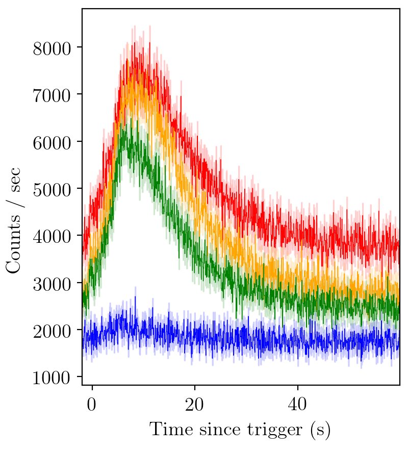
BATSE trigger 7475
Say we would like to fit a GRB light-curve such as the above, and determine its pulse parameters. First we must load the relevant modules.
from PyGRB.main.fitpulse import PulseFitter
from PyGRB.backend.makemodels import create_model_from_key
The PulseFitter class is the main workhorse of the software.
GRB = PulseFitter(7475, times = (-2, 60),
          datatype = 'discsc', nSamples = 200, sampler = 'nestle',
          priors_pulse_start = -5, priors_pulse_end = 30)
The first argument specifies the BATSE trigger to be analysed, in this case trigger 7475.
Times can either be specified as ‘T90’, ‘full’, or a tuple of start and end times.
In the case of trigger 7475, most of the action happens over about (-2, 60), so we choose this interval for our times.
The nSamples parameter determines how many live points the nested sampler is initiated with.
The sampler parameter is used to choose between samplers.
The priors_pulse_start and priors_pulse_end parameters are used to set the (uniform) interval over which the program will allow the pulse start times.
The datatype parameter specifies which kind of data we would like to download and analyse.
Typically ‘discsc’ is the most useful.
‘tte’ is better for short GRBs.
The data will be downloaded and stored in data/.
create_model_from_key allows us to specify pulse models based on a simple key. The simple pulse type, a fast-rise exponential-decay (FRED) pulse, is utilised by
key = 'F'
model = create_model_from_key(key)
Finally, we run the model through the sampler
GRB.main_multi_channel(channels = [0, 1, 2, 3], model = model)
The data products are stored in products/.
The complete script for the above tutorial is here:
from PyGRB.main.fitpulse import PulseFitter
from PyGRB.backend.makemodels import create_model_from_key

GRB = PulseFitter(7475, times = (-2, 60),
          datatype = 'discsc', nSamples = 200, sampler = 'nestle',
          priors_pulse_start = -10, priors_pulse_end = 30, p_type ='docs')

key = 'F'
model = create_model_from_key(key)
GRB.main_multi_channel(channels = [0, 1, 2, 3], model = model)
Something like the following will be printed to the console:
18:55 bilby INFO    : Single likelihood evaluation took 4.089e-04 s
18:55 bilby INFO    : Using sampler Nestle with kwargs {'method': 'multi', 'npoints': 200, 'update_interval': None, 'npdim': None, 'maxiter': None, 'maxcall': None, 'dlogz': None, 'decline_factor': None, 'rstate': None, 'callback': <function print_progress at 0x00000185F8598AE8>, 'steps': 20, 'enlarge': 1.2}
it=  6048 logz=-4174.731348
18:55 bilby INFO    : Sampling time: 0:00:15.464772
18:55 bilby INFO    : Summary of results:
nsamples: 6249
log_noise_evidence:    nan
log_evidence: -4174.477 +/-  0.368
log_bayes_factor:    nan +/-  0.368
The total number of posterior samples, nsamples, in this instance is 6249. This is the length of posterior chains accessed through the code block at the bottom of this page. The log_noise_evidence is used for Bilby’s gravitational wave inference. It is irrelevant for PyGRB, as PyGRB’s Poisson likelihood does not specify an additional noise model. The log_evidence is the Bayesian evidence in support of this data given the specified model. The Bayes factor is the comparison of evidence between two models. Here, log_bayes_factor is NaN as there is only one model specified, and the comparison cannot be made. PyGRB does it’s model comparison external to the inbuilt Bilby functionality.
Errors like the following can be ignored.
RuntimeWarning: overflow encountered in multiply ...
They are bad evaluations of the likelihood and have no real effect on the results. In the unlikely event that they happen consistently, it may mean that the sampler is stuck in a bad region of parameter space. Restarting the sampler for that particular evaluation should fix the problem.
This will create three sets of files in the products directory.
Nested sampling posterior chains, which are stored as JSON files.
Corner plots of the posteriors.
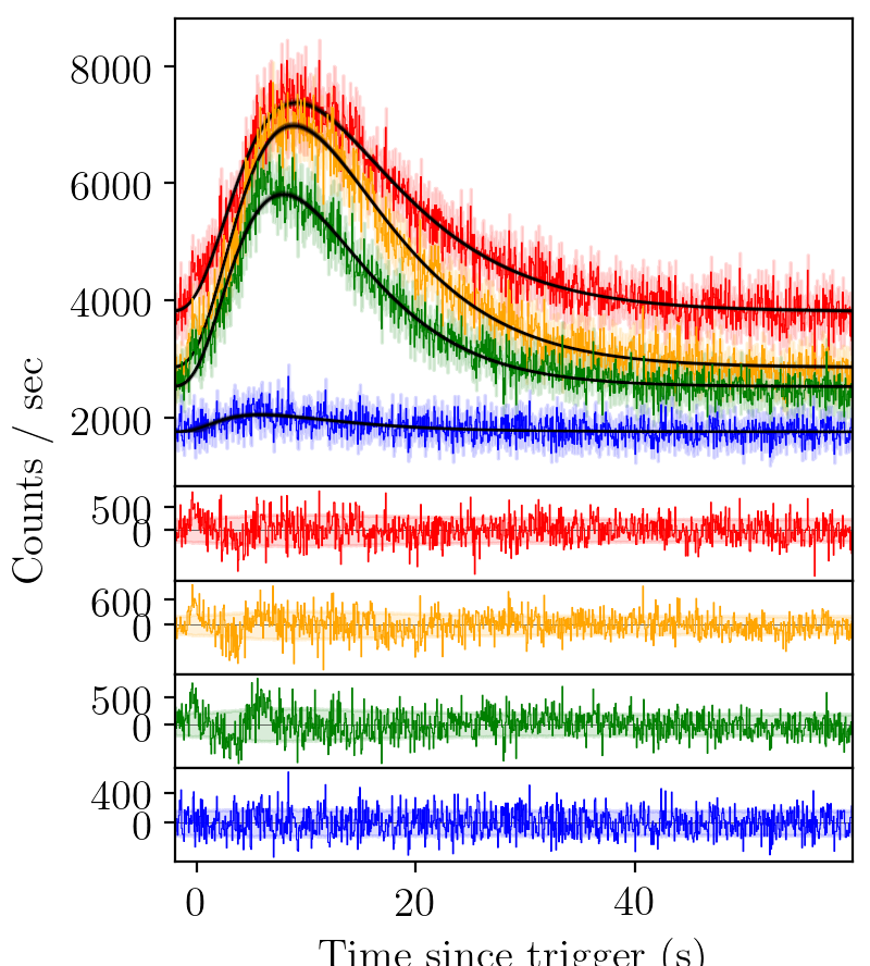
Higher data products, the light-curves of each of the individual channels. These include by default analysis of the light-curve fit residuals to test for goodness-of-fit.
These are put into subdirectories based on the trigger number and the number of live points. Files for this example can be found under /products/7475_model_comparison_200/.
BATSE trigger 7475 with FRED fit
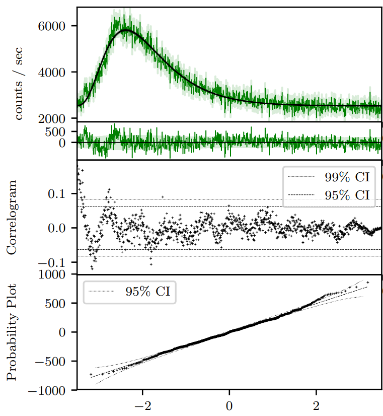
BATSE trigger 7475 with FRED pulse fit on a single channel (channel 3). The green shaded regions are the 1-sigma statistical (Poisson) uncertainty. The correlogram is a visualisation of the autocorrelation of the residuals in the second panel. For a “good” fit, one expects 95% (99%) of the points to lie within the 95% (99%) confidence intervals. It is interesting to note in this case there is a sinusoidal structure all the way to the end of the pulse, even though the deviations from the fit are not large. The probability plot tests the divergence of the residuals from zero for normality. Again we see that the residuals are normally distributed to a good approximation.
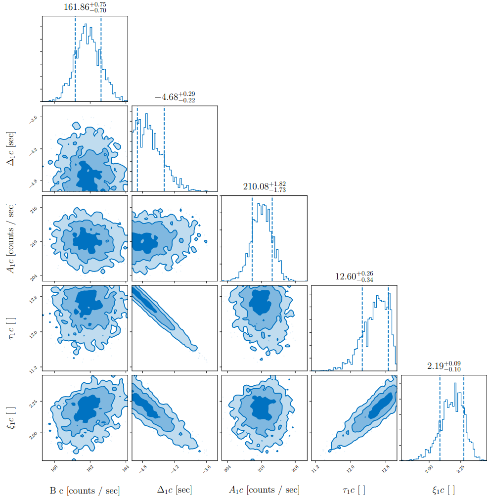
BATSE trigger 7475 with FRED pulse fit on a single channel (channel 3) posterior corner plot. The parameter space is undersampled, (the posterior histograms are patchy), but that does not matter since this tutorial is for illustrative purposes only.
In answer to our initial question, pulse parameters may be read straight of the posterior distribution (or accessed through the posterior chain JSON file).
The following code block could be appended to the end of basic.py
# pick a channel to analyse
channel = 0

# create the right filename to open
result_label = f'{GRB.fstring}{GRB.clabels[channel]}'
open_result  = f'{GRB.outdir}/{result_label}_result.json'
result = bilby.result.read_in_result(filename=open_result)

# channel 0 parameters are subscripted with _a
parameter = 'background_a'

# the posterior samples are accessed through the result object
posterior_samples = result.posterior[parameter].values

# to find the median
import numpy as np
posterior_samples_median = np.median(posterior_samples)